
TOOLS and FUNCTIONS for VEM JDE Used in different versions of VEM
pyhrf.vbjde.vem_tools.A_Entropy(Sigma_A, M, J)¶pyhrf.vbjde.vem_tools.Compute_FreeEnergy(y_tilde, m_A, Sigma_A, mu_Ma, sigma_Ma, m_H, Sigma_H, AuxH, R, R_inv, sigmaH, sigmaG, m_C, Sigma_C, mu_Mc, sigma_Mc, m_G, Sigma_G, AuxG, q_Z, neighboursIndexes, Beta, Gamma, gamma, gamma_h, gamma_g, sigma_eps, XX, W, J, D, M, N, K, hyp, Gamma_X, Gamma_WX, plot=False, bold=False, S=1)¶pyhrf.vbjde.vem_tools.H_Entropy(Sigma_H, D)¶pyhrf.vbjde.vem_tools.PolyMat(Nscans, paramLFD, tr)¶Build polynomial basis
pyhrf.vbjde.vem_tools.Q_Entropy(q_Z, M, J)¶pyhrf.vbjde.vem_tools.Q_expectation_Ptilde(q_Z, neighboursIndexes, Beta, gamma, K, M)¶pyhrf.vbjde.vem_tools.RF_Entropy(Sigma_RF, D)¶pyhrf.vbjde.vem_tools.RF_expectation_Ptilde(m_X, Sigma_X, sigmaX, R, R_inv, D)¶pyhrf.vbjde.vem_tools.RL_Entropy(Sigma_RL, M, J)¶pyhrf.vbjde.vem_tools.RL_expectation_Ptilde(m_X, Sigma_X, mu_Mx, sigma_Mx, q_Z)¶pyhrf.vbjde.vem_tools.Z_Entropy(q_Z, M, J)¶pyhrf.vbjde.vem_tools.beta_gradient(beta, labels_proba, labels_neigh, neighbours_indexes, gamma, gradient_method='m1')¶Computes the gradient of the beta function.
The maximization of  needs the computation of its derivative with respect to
  .
.
Method 1
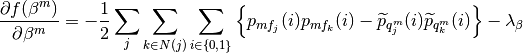
Method 2
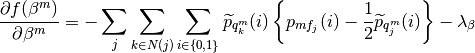
where
| Parameters: | |
|---|---|
| Returns: | gradient – the gradient estimated in beta |
| Return type: |
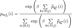
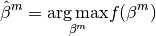
pyhrf.vbjde.vem_tools.beta_maximization(beta, labels_proba, neighbours_indexes, gamma)¶Computes the Beta Maximization step of the JDE VEM algorithm.
The maximization over each corresponds to the M-step obtained for a standard Hiddden MRF model:
| Parameters: |
|
|---|---|
| Returns: |
|
Notes
See beta_gradient() function.
pyhrf.vbjde.vem_tools.buildFiniteDiffMatrix(order, size, regularization=None)¶Build the finite difference matrix used for the hrf regularization prior.
| Parameters: | |
|---|---|
| Returns: | diffMat – the finite difference matrix |
| Return type: | ndarray, shape (size, size) |
pyhrf.vbjde.vem_tools.computeFit(hrf_mean, nrls_mean, X, nb_voxels, nb_scans)¶Compute the estimated induced signal by each stimulus.
| Parameters: |
|
|---|---|
| Returns: | |
| Return type: | ndarray |
pyhrf.vbjde.vem_tools.computeFit_asl(H, m_A, G, m_C, W, XX)¶Compute Fit
pyhrf.vbjde.vem_tools.compute_contrasts(condition_names, contrasts, m_A, m_C, Sigma_A, Sigma_C, M, J)¶pyhrf.vbjde.vem_tools.compute_mat_X_2(nbscans, tr, lhrf, dt, onsets, durations=None)¶pyhrf.vbjde.vem_tools.constraint_norm1_b(Ftilde, Sigma_F, positivity=False, perfusion=None)¶Constrain with optimization strategy
pyhrf.vbjde.vem_tools.contrasts_mean_var_classes(contrasts, condition_names, nrls_mean, nrls_covar, nrls_class_mean, nrls_class_var, nb_contrasts, nb_classes, nb_voxels)¶Computes the contrasts nrls from the conditions nrls and the mean and variance of the gaussian classes of the contrasts (in the cases of all inactive conditions and all active conditions).
| Parameters: |
|
|---|---|
| Returns: |
|
pyhrf.vbjde.vem_tools.cosine_drifts_basis(nb_scans, param_lfd, tr)¶Build cosine drifts basis.
| Parameters: | |
|---|---|
| Returns: | drifts_basis – K is determined by the scipy.linalg.orth function and corresponds to the effective rank of the matrix it is applied to (see function’s docstring) |
| Return type: | ndarray, shape (nb_scans, K) |
pyhrf.vbjde.vem_tools.covariance_matrix(order, D, dt)¶pyhrf.vbjde.vem_tools.create_conditions(onsets, durations, nb_conditions, nb_scans, hrf_len, tr, dt)¶Generate the occurrences matrix.
| Parameters: |
|
|---|---|
| Returns: |
|
pyhrf.vbjde.vem_tools.create_neighbours(graph)¶Transforms the graph list in ndarray. This is for performances purposes. Sets the empty neighbours to -1.
| Parameters: | graph (list of ndarray) – each graph[i] represents the list of neighbours of the ith voxel |
|---|---|
| Returns: | neighbours_indexes |
| Return type: | ndarray |
pyhrf.vbjde.vem_tools.drifts_coeffs_fit(signal, drift_basis)¶# TODO
| Parameters: |
|
|---|---|
| Returns: | drift_coeffs |
| Return type: | ndarray, shape |
pyhrf.vbjde.vem_tools.expectation_A_asl(H, G, m_C, W, XX, Gamma, Gamma_X, q_Z, mu_Ma, sigma_Ma, J, y_tilde, Sigma_H, sigma_eps_m)¶Expectation-A step:
![p_A = argmax_h(E_pc,pq,ph,pg[log p(a|y, h, c, g, q; theta)]) \propto exp(E_pc,ph,pg[log p(y|h, a, c, g; theta)] + E_pq[log p(a|q; mu_Ma, sigma_Ma)])](../_images/math/4993891819359d7f3b108259fa11acb1e9be7af5.png)
| Returns: | |
|---|---|
| Return type: | m_A, Sigma_A of probability distribution p_A of the current iteration |
pyhrf.vbjde.vem_tools.expectation_A_ms(m_A, Sigma_A, H, G, m_C, W, XX, Gamma, Gamma_X, q_Z, mu_Ma, sigma_Ma, J, y_tilde, Sigma_H, sigma_eps_m, N, M, D, S)¶Expectation-A step:
| Returns: | |
|---|---|
| Return type: | m_A, Sigma_A of probability distribution p_A of the current iteration |
pyhrf.vbjde.vem_tools.expectation_C_asl(G, H, m_A, W, XX, Gamma, Gamma_X, q_Z, mu_Mc, sigma_Mc, J, y_tilde, Sigma_G, sigma_eps_m)¶Expectation-C step:
![p_C = argmax_h(E_pa,pq,ph,pg[log p(a|y, h, a, g, q; theta)]) \propto exp(E_pa,ph,pg[log p(y|h, a, c, g; theta)] + E_pq[log p(c|q; mu_Mc, sigma_Mc)])](../_images/math/239d6f6a797a5ef1b6ae927efcfc6a0360ccadf2.png)
| Returns: | |
|---|---|
| Return type: | m_C, Sigma_C of probability distribution p_C of the current iteration |
pyhrf.vbjde.vem_tools.expectation_C_ms(m_C, Sigma_C, G, H, m_A, W, XX, Gamma, Gamma_X, q_Z, mu_Mc, sigma_Mc, J, y_tilde, Sigma_G, sigma_eps_m, N, M, D, S)¶Expectation-C step:
| Returns: | |
|---|---|
| Return type: | m_C, Sigma_C of probability distribution p_C of the current iteration |
pyhrf.vbjde.vem_tools.expectation_G_asl(Sigma_C, m_C, m_A, H, XX, W, WX, Gamma, Gamma_WX, XW_Gamma_WX, J, y_tilde, cov_noise, R_inv, sigmaG, prior_mean_term, prior_cov_term)¶Expectation-G step:
![p_G = argmax_g(E_pa,pc,ph[log p(g|y, a, c, h; theta)]) \propto exp(E_pa,pc,ph[log p(y|h, a, c, g; theta) + log p(g; sigmaG)])](../_images/math/27fe0df1bfecc8c35fbb33e2c8a4306296cdcbf3.png)
| Returns: | |
|---|---|
| Return type: | m_G, Sigma_G of probability distribution p_G of the current iteration |
pyhrf.vbjde.vem_tools.expectation_G_ms(Sigma_C, m_C, m_A, H, XX, W, WX, Gamma, Gamma_WX, XW_Gamma_WX, J, y_tilde, cov_noise, R_inv, sigmaG, prior_mean_term, prior_cov_term, N, M, D, S)¶Expectation-G step:
| Returns: | |
|---|---|
| Return type: | m_G, Sigma_G of probability distribution p_G of the current iteration |
pyhrf.vbjde.vem_tools.expectation_H_asl(Sigma_A, m_A, m_C, G, XX, W, Gamma, Gamma_X, X_Gamma_X, J, y_tilde, cov_noise, R_inv, sigmaH, prior_mean_term, prior_cov_term)¶Expectation-H step:
![p_H = argmax_h(E_pa,pc,pg[log p(h|y, a, c, g; theta)]) \propto exp(E_pa,pc,pg[log p(y|h, a, c, g; theta) + log p(h; sigmaH)])](../_images/math/bbd71b37d2268b71bff1dff520739c1ef9fa4f45.png)
| Returns: | |
|---|---|
| Return type: | m_H, Sigma_H of probability distribution p_H of the current iteration |
pyhrf.vbjde.vem_tools.expectation_H_ms(Sigma_A, m_A, m_C, G, XX, W, Gamma, Gamma_X, X_Gamma_X, J, y_tilde, cov_noise, R_inv, sigmaH, prior_mean_term, prior_cov_term, N, M, D, S)¶Expectation-H step:
| Returns: | |
|---|---|
| Return type: | m_H, Sigma_H of probability distribution p_H of the current iteration |
pyhrf.vbjde.vem_tools.expectation_H_ms_concat(Sigma_A, m_A, m_C, G, XX, W, Gamma, Gamma_X, X_Gamma_X, J, y_tilde, cov_noise, R_inv, sigmaH, prior_mean_term, prior_cov_term, S)¶Expectation-H step:
| Returns: | |
|---|---|
| Return type: | m_H, Sigma_H of probability distribution p_H of the current iteration |
pyhrf.vbjde.vem_tools.expectation_Ptilde_Likelihood(y_tilde, m_A, Sigma_A, H, Sigma_H, m_C, Sigma_C, G, Sigma_G, XX, W, sigma_eps, Gamma, J, D, M, N, Gamma_X, Gamma_WX)¶pyhrf.vbjde.vem_tools.expectation_Q_asl(Sigma_A, m_A, Sigma_C, m_C, sigma_Ma, mu_Ma, sigma_Mc, mu_Mc, Beta, p_q_t, p_Q, neighbours_indexes, graph, M, J, K)¶pyhrf.vbjde.vem_tools.expectation_Q_async_asl(Sigma_A, m_A, Sigma_C, m_C, sigma_Ma, mu_Ma, sigma_Mc, mu_Mc, Beta, p_q_t, p_Q, neighbours_indexes, graph, M, J, K)¶pyhrf.vbjde.vem_tools.expectation_Q_ms(Sigma_A, m_A, Sigma_C, m_C, sigma_Ma, mu_Ma, sigma_Mc, mu_Mc, Beta, p_q_t, p_Q, neighbours_indexes, graph, M, J, K, S)¶pyhrf.vbjde.vem_tools.expectation_ptilde_hrf(hrf_mean, hrf_covar, sigma_h, hrf_regu_prior, hrf_regu_prior_inv, hrf_len)¶Expectation with respect to p_tilde hrf.
![\mathrm{E}_{\widetilde{p}_{h}}\left[ \log p(h | \sigma_{h}) \right] = -\frac{D+1}{2}\log 2\pi -
\frac{D-1}{2}\log \sigma_{h} - \frac{\log \left| \mathbf{R} \right|}{2} - \frac{m^{t}_{h}\mathbf{R}^{-1}m_{h}
+ \mathrm{tr} \left( \Sigma_{h} \mathbf{R}^{-1} \right)}{2 \sigma_{h}}](../_images/math/a75c61ccc850b8e8a32fac3fe105370c46c17a94.png)
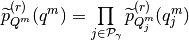
pyhrf.vbjde.vem_tools.expectation_ptilde_labels(labels_proba, neighbours_indexes, beta, nb_conditions, nb_classes)¶Expectation with respect to p_tilde q (or z).
![\mathrm{E}_{\widetilde{p}_{q}} \left[ \log p (q | \beta ) \right] = \sum\limits_{m} & \left\{
- \sum\limits_{j} \left\{ \log \left( \sum\limits^{1}_{i=0} \exp \left(
\beta^{m} \sum\limits_{k \in N(j)} \widetilde{p}_{q^{m}_{k}} (i) \right)
\right) \right\} \right. \\
& \left. - \beta^{m} \sum\limits_{j}\sum\limits_{k \in N(j)}\sum\limits^{1}_{i=0}
\left[ p^{MF}_{j}(i) \left( \frac{p^{MF}_{k}(i)}{2} -
\widetilde{p}_{q^{m}_{k}} (i) \right) -
\frac{1}{2}\widetilde{p}_{q^{m}_{j}}(i)\widetilde{p}_{q^{m}_{k}}(i) \right]
\right\}](../_images/math/f2629b4a8bbb7fc2a4e8113106e32a57dee44d10.png)
pyhrf.vbjde.vem_tools.expectation_ptilde_likelihood(data_drift, nrls_mean, nrls_covar, hrf_mean, hrf_covar, occurence_matrix, noise_var, noise_struct, nb_voxels, nb_scans)¶Expectation with respect to likelihood.
![\mathrm{E}_{\widetilde{p}_{a}\widetilde{p}_{h}\widetilde{p}_{q}}\left[\log p(y | a,h,q; \theta) \right] =
-\frac{NJ}{2} \log 2\pi + \frac{J}{2}\log\left| \Lambda_{j} \right| - N\sum\limits_{j \in J}\log
v_{b_{j}} + \frac{1}{2v_{b_{j}}}\sum\limits_{j \in J}V_{j}](../_images/math/01b6a6eaaee7393f993c356ddaf12e8e1d8fd557.png)
where

| Parameters: |
|
|---|---|
| Returns: | ptilde_likelihood |
| Return type: |
pyhrf.vbjde.vem_tools.expectation_ptilde_nrls(labels_proba, nrls_class_mean, nrls_class_var, nrls_mean, nrls_covar)¶Expectation with respect to p_tilde a.
![\mathrm{E}_{\widetilde{p}_{a}\widetilde{p}_{q}}[\log p (a | q, \theta_{a})] = \sum\limits_{m}\sum\limits_{j}
& \left\{ \left[1 - \widetilde{p}_{q^{m}_{j}}(1) \right] \left[\log\frac{1}{\sqrt{2\pi\sigma^{2m}_{0}}} -
\frac{\left(m_{a^{m}_{j}} - \mu^{m}_{0} \right)^{2} + \Sigma_{a^{m,m}_{j}}}{2\sigma^{2m}_{0}} \right] +
\right. \\ & \left. \widetilde{p}_{q^{m}_{j}}(1) \left[\log\frac{1}{\sqrt{2\pi\sigma^{2m}_{1}}} -
\frac{\left(m_{a^{m}_{j}} - \mu^{m}_{1} \right)^{2} + \Sigma_{a^{m,m}_{j}}}{2\sigma^{2m}_{1}} \right] \right\}](../_images/math/a9fc248f27f53d904b7812db1e76bb7501f2b898.png)
pyhrf.vbjde.vem_tools.fit_hrf_two_gammas(hrf_mean, dt, duration)¶Fits the estimated HRF to the standard two gammas model.
| Parameters: | |
|---|---|
| Returns: |
|
pyhrf.vbjde.vem_tools.free_energy_computation(nrls_mean, nrls_covar, hrf_mean, hrf_covar, hrf_len, labels_proba, data_drift, occurence_matrix, noise_var, noise_struct, nb_conditions, nb_voxels, nb_scans, nb_classes, nrls_class_mean, nrls_class_var, neighbours_indexes, beta, sigma_h, hrf_regu_prior, hrf_regu_prior_inv, gamma, hrf_hyperprior)¶Compute the free energy functional.
![\mathcal{F}(q, \theta) = \mathrm{E}_{q}\left[ \log p(y, A, H, Z ; \theta) \right] + \mathcal{G}(q)](../_images/math/9d17d4706b43c4a8c8743755db80a5c2e6b79abe.png)
where ![E_{q}[\cdot]](../_images/math/17cd6f4b8c4f0af9829f6a7462156588833cb157.png) denotes the expectation with respect to q and
denotes the expectation with respect to q and
 is the entropy of q.
| Returns: | free_energy |
|---|---|
| Return type: | float |
pyhrf.vbjde.vem_tools.fun(Beta, p_Q, Qtilde_sumneighbour, neighboursIndexes, gamma)¶function to minimize
pyhrf.vbjde.vem_tools.grad_fun(Beta, p_Q, Qtilde_sumneighbour, neighboursIndexes, gamma)¶function to minimize
pyhrf.vbjde.vem_tools.hrf_entropy(hrf_covar, hrf_len)¶Compute the entropy of the hemodynamic response function. The entropy of a multivariate normal distribution is
where n is the dimensionality of the vector space and  is the determinant of the
covariance matrix.
is the determinant of the
covariance matrix.
| Parameters: |
|
|---|---|
| Returns: | entropy |
| Return type: |
pyhrf.vbjde.vem_tools.hrf_expectation(nrls_covar, nrls_mean, occurence_matrix, noise_struct, hrf_regu_prior_inv, sigmaH, nb_voxels, y_tilde, noise_var, prior_mean_term=0.0, prior_cov_term=0.0)¶Computes the VE-H step of the JDE-VEM algorithm.
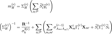
where
Here,  and
and  denote the
 and
and  entries of the mean vector and covariance matrix of the current
 , respectively.
| Parameters: |
|
|---|---|
| Returns: |
|
pyhrf.vbjde.vem_tools.labels_entropy(labels_proba)¶Compute the labels entropy.
| Parameters: | labels_proba (ndarray, shape (nb_conditions, nb_classes, nb_voxels)) – Probability of each voxel to be in one class |
|---|---|
| Returns: | entropy |
| Return type: | float |
pyhrf.vbjde.vem_tools.labels_expectation(nrls_covar, nrls_mean, nrls_class_var, nrls_class_mean, beta, labels_proba, neighbours_indexes, nb_conditions, nb_classes, nb_voxels=None, parallel=True, nans_init=False)¶Computes the E-Z (or E-Q) step of the JDE-VEM algorithm.
Using the mean-field approximation,
 is approximated by a factorized density
 such that if
 , then
  where
where  is a particular configuration of
 updated at each iteration according to a specific scheme and
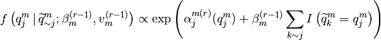
where
![\left\{ \alpha^{m(r)}_{j} = \left( -v^{(r)}_{A_{j}^{m}A^{m''}_{j}} \left[ \frac{1}{v^{(r-1)}_{0m}},
\frac{1}{v^{(r-1)}_{1m}} \right] \right)^{t}, j \in \mathcal{P}_{\gamma}\right\}](../_images/math/eab50416c3805c5c5ec3cf59f0e70dc228b4f682.png)
and  denotes the
  entries of the covariance matrix

Notes
The mean-field fixed point equation is defined in:
Celeux, G., Forbes, F., & Peyrard, N. (2003). EM procedures using mean field-like approximations for Markov model-based image segmentation. Pattern Recognition, 36(1), 131–144. https://doi.org/10.1016/S0031-3203(02)00027-4
| Parameters: |
|
|---|---|
| Returns: | labels_proba |
| Return type: | ndarray, shape (nb_conditions, nb_classes, nb_voxels) |
pyhrf.vbjde.vem_tools.maximization_LA_asl(Y, m_A, m_C, XX, WP, W, WP_Gamma_WP, H, G, Gamma)¶pyhrf.vbjde.vem_tools.maximization_Mu_asl(H, G, matrix_covH, matrix_covG, sigmaH, sigmaG, sigmaMu, Omega, R_inv)¶pyhrf.vbjde.vem_tools.maximization_beta_m2_asl(beta, p_Q, Qtilde_sumneighbour, Qtilde, neighboursIndexes, maxNeighbours, gamma, MaxItGrad, gradientStep)¶pyhrf.vbjde.vem_tools.maximization_beta_m2_scipy_asl(Beta, p_Q, Qtilde_sumneighbour, Qtilde, neighboursIndexes, maxNeighbours, gamma, MaxItGrad, gradientStep)¶Maximize beta
pyhrf.vbjde.vem_tools.maximization_beta_m4_asl(beta, p_Q, Qtilde_sumneighbour, Qtilde, neighboursIndexes, maxNeighbours, gamma, MaxItGrad, gradientStep)¶pyhrf.vbjde.vem_tools.maximization_class_proba(labels_proba, nrls_mean, nrls_covar)¶Computes the M-(mu, sigma) step of the JDE-VEM algorithm.
pyhrf.vbjde.vem_tools.maximization_drift_coeffs(data, nrls_mean, occurence_matrix, hrf_mean, noise_struct, drift_basis)¶Computes the M-(l, Gamma) step of the JDE-VEM algorithm. In the AR(1) case:
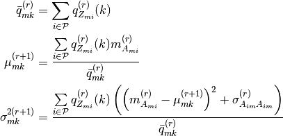
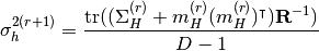
pyhrf.vbjde.vem_tools.maximization_mu_sigma_asl(q_Z, m_X, Sigma_X)¶pyhrf.vbjde.vem_tools.maximization_mu_sigma_ms(q_Z, m_X, Sigma_X, M, J, S, K)¶pyhrf.vbjde.vem_tools.maximization_noise_var(occurence_matrix, hrf_mean, hrf_covar, nrls_mean, nrls_covar, noise_struct, data_drift, nb_scans)¶Computes the M-sigma_epsilon step of the JDE-VEM algorithm.
![\sigma^{2(r)}_{j} = \frac{1}{N} \left(\mathrm{E}_{\widetilde{p}^{(r)}_{A_{j}}} \left[a^{t}_{j}
\widetilde{\Lambda}^{(r)}_{j} a_{j} \right] - 2 \left(m^{(r)}_{A_{j}}\right)^{t} \widetilde{G}^{(r)}_{j}
y^{(r)}_{j} + \left(y^{(r)}_{j}\right)^{t} \Lambda^{(r)}_{j}y^{(r)}_{j} \right)](../_images/math/8e654c4479ed584b71674fd6daa2aca90add4f86.png)
where matrix ![\widetilde{\Lambda}^{(r)}_{j} = \mathrm{E}_{\widetilde{p}^{(r)}_{H}}
\left[ G^{t}\Lambda^{(r)}_{j}G \right]](../_images/math/7abd048a0e146ec636f3a4bba79e4694813d75d6.png) is a
is a  whose element
  is given by
pyhrf.vbjde.vem_tools.maximization_sigmaH(D, Sigma_H, R, m_H)¶Computes the M-sigma_h step of the JDE-VEM algorithm.
pyhrf.vbjde.vem_tools.maximization_sigmaH_prior(D, Sigma_H, R, m_H, gamma_h)¶Computes the M-sigma_h step of the JDE-VEM algorithm with a prior.
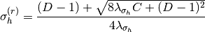
where
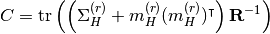
pyhrf.vbjde.vem_tools.maximization_sigma_asl(D, Sigma_H, R_inv, m_H, use_hyp, gamma_h)¶pyhrf.vbjde.vem_tools.maximization_sigma_noise_asl(XX, m_A, Sigma_A, H, m_C, Sigma_C, G, Sigma_H, Sigma_G, W, y_tilde, Gamma, Gamma_X, Gamma_WX, N)¶Maximization sigma_noise
pyhrf.vbjde.vem_tools.maximum(iterable)¶Return the maximum and the indice of the maximum of an iterable.
| Parameters: | iterable (iterable or numpy array) – |
|---|---|
| Returns: |
|
pyhrf.vbjde.vem_tools.mult(v1, v2)¶Multiply two vectors.
The first vector is made vertical and the second one horizontal. The result will be a matrix of size len(v1), len(v2).
| Parameters: |
|
|---|---|
| Returns: | x |
| Return type: | ndarray, shape (len(v1), len(v2)) |
pyhrf.vbjde.vem_tools.norm1_constraint(function, variance)¶Returns the function constrained with optimization strategy.
| Parameters: |
|
|---|---|
| Returns: | optimized_function |
| Return type: | numpy array |
| Raises: |
|
pyhrf.vbjde.vem_tools.normpdf(x, mu, sigma)¶pyhrf.vbjde.vem_tools.nrls_entropy(nrls_covar, nb_conditions)¶Compute the entropy of neural response levels. The entropy of a multivariate normal distribution is
where n is the dimensionality of the vector space and is the determinant of the
covariance matrix.
| Parameters: |
|
|---|---|
| Returns: | entropy |
| Return type: |
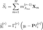
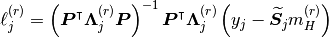
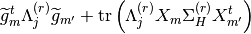
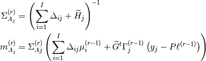
pyhrf.vbjde.vem_tools.nrls_expectation(hrf_mean, nrls_mean, occurence_matrix, noise_struct, labels_proba, nrls_class_mean, nrls_class_var, nb_conditions, y_tilde, nrls_covar, hrf_covar, noise_var)¶Computes the VE-A step of the JDE-VEM algorithm.
where:
The mth column of  is denote by
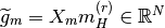
![\Delta_{ij} &= \mathrm{diag}_{M}\left[\frac{q^{(r-1)}_{Z_{mj}}(i)}{\sigma^{2(r)}_{mi}}\right] \\
\widetilde{H}_{j} &= \widetilde{g}^{t}_{m} \Gamma^{(r-1)}_{j} \widetilde{g}_{m'} + \mathrm{tr}\left( \Gamma^{(r-1)}_{j}X_{m} \Sigma^{(r)}_{H}X^{t}_{m'} \right)](../_images/math/252eda09b3aa0edcd41344089f568954c72f86fe.png)
| Parameters: |
|
|---|---|
| Returns: |
|
pyhrf.vbjde.vem_tools.plot_convergence(ni, M, cA, cC, cH, cG, cAH, cCG, SUM_q_Z, mua1, muc1, FE)¶pyhrf.vbjde.vem_tools.plot_response_functions_it(ni, NitMin, M, H, G, Mu=None, prior=None)¶pyhrf.vbjde.vem_tools.polyFit(signal, tr, order, p)¶pyhrf.vbjde.vem_tools.poly_drifts_basis(nb_scans, param_lfd, tr)¶Build polynomial drifts basis.
| Parameters: | |
|---|---|
| Returns: | drifts_basis – K is determined by the scipy.linalg.orth function and corresponds to the effective rank of the matrix it is applied to (see function’s docstring) |
| Return type: | ndarray, shape (nb_scans, K) |
pyhrf.vbjde.vem_tools.ppm_contrasts(contrasts_mean, contrasts_var, contrasts_class_mean, contrasts_class_var, threshold_a='std_inact', threshold_g=0.95)¶Computes the ppm for the given contrast using either the standard deviation of the “all inactive conditions” class gaussian (default) or the intersection of the [all inactive conditions] and [all active conditions] classes gaussians as threshold for the PPM_a and 0.95 (default) for the PPM_g. Be carefull, this computation considers the mean of the inactive class as zero.
| Parameters: |
|
|---|---|
| Returns: |
|
pyhrf.vbjde.vem_tools.ppms_computation(elements_mean, elements_var, class_mean, class_var, threshold_a='std_inact', threshold_g=0.9)¶Considering the elements_mean and elements_var from a gaussian distribution, commutes the posterior probability maps considering for the alpha threshold, either the standard deviation of the [all inactive conditions] gaussian class or the intersection of the [all (in)active conditions] gaussian classes; and for the gamma threshold 0.9 (default).
The posterior probability maps (PPM) per experimental condition is computed as
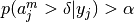 . Note that we have to thresholds to set. We set
  to get
a posterior probability distribution, and
to get
a posterior probability distribution, and  is the threshold that we set to see a certain level of
significance. As default, we chose a threshold for each experimental condition m as the
intersection of the two Gaussian densities of the Gaussian Mixture Model (GMM) that represent active and non-active
voxel.
is the threshold that we set to see a certain level of
significance. As default, we chose a threshold for each experimental condition m as the
intersection of the two Gaussian densities of the Gaussian Mixture Model (GMM) that represent active and non-active
voxel.
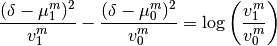
 and
and  being the parameters of the GMM in
  corresponding to
active (i=0) and non-active (i=1) voxels for experimental condition m.
corresponding to
active (i=0) and non-active (i=1) voxels for experimental condition m.
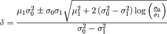
Be careful, this computation considers the mean of the inactive class as zero.
Notes
nb_elements refers either to the number of contrasts (for the PPMs contrasts computation) or for the number of conditions (for the PPMs nrls computation).
| Parameters: |
|
|---|---|
| Returns: |
|
pyhrf.vbjde.vem_tools.roc_curve(dvals, labels, rocN=None, normalize=True)¶Compute ROC curve coordinates and area
returns (FP coordinates, TP coordinates, AUC )
pyhrf.vbjde.vem_tools.sum_over_neighbours(neighbours_indexes, array_to_sum)¶Sums the array_to_sum over the neighbours in the graph.